
새로새록
python - opencv: 사진 윤곽선 기본(2) 본문
import cv2
import numpy as np
import matplotlib.pyplot as plt

image = np.full((512, 512, 3), 255, np.uint8)
image = cv2.line(image, (0, 0), (255, 255), (255, 0, 0), 3)

plt.imshow(image)
plt.show()
도형그리기
선그리기
import cv2
import numpy as np
import matplotlib.pyplot as plt

image = np.full((512, 512, 3), 255, np.unit8)
image = cv2.rectangle(image, (20,20), (255,255), (255,0,0), 3)

plt.imshow(image)
plt.show()
직사각형
import cv2
import numpy as np
import matplotlib.pyplot as plt

image = np.full((512,512,3), 255, np.unit8)
image = cv2.circle(image, (255,255), 30, (255,0,0), 3)

plt.imshow(image)
plt.show()
원
import cv2
import numpy as np
import matplotlib.pyplot as plt

image = np.full((512, 512, 3), 255, np.uint8)
points = np.array([[5, 5], [128, 258], [483, 444], [400, 150]])
image = cv2.polylines(image, [points], True, (0, 0, 255), 4)

plt.imshow(image)
plt.show()
사각형
import cv2
import numpy as np
import matplotlib.pyplot as plt

image = np.full((512, 512, 3), 255, np.uint8)
image = cv2.putText(image, 'Hello World', (0, 200), cv2.FONT_ITALIC, 2, (255, 0, 0))

plt.imshow(image)
plt.show()
텍스트
윤곽선그리기
cv2.findContours(image, mode, method): 이미지에서 Contour들을 찾는 함수
mode: Contour들을 찾는 방법
1) RETR_EXTERNAL: 바깥쪽 Line만 찾기
2) RETR_LIST: 모든 Line을 찾지만, Hierarchy 구성 X
3) RETR_TREE: 모든 Line을 찾으며, 모든 Hierarchy 구성
Omethod: Contour들을 찾는 근사치 방법
1) CHAIN_APPROX_NONE: 모든 Contour 포인트 저장
2) CHAIN_APPROX_SIMPLE: Contour Line을 그릴 수 있는 포인트만 저장
입력 이미지는 Gray Scale Threshold 전처리 과정이 필요합니다.
cv2.drawContours(image, contours, contour_index, color, thickness):
Contour들을 그리는 함수
contour_index: 그리고자 하는 Contours Line (전체: -1)
import cv2
import numpy as np
import matplotlib.pyplot as plt
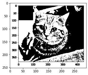
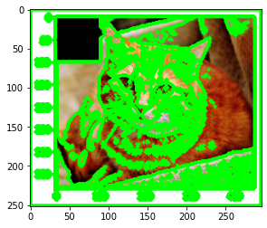
image = cv2.imread('Downloads/cat.png')
image_gray = cv2.cvtColor(image, cv2.COLOR_BGR2GRAY)
ret, thresh = cv2.threshold(image_gray, 127, 255, 0)
plt.imshow(cv2.cvtColor(thresh, cv2.COLOR_GRAY2RGB))
plt.show()
contours, _ = cv2.findContours(thresh, cv2.RETR_TREE, cv2.CHAIN_APPROX_SIMPLE)
image1 = cv2.drawContours(image, contours, -1, (0, 255, 0), 4)
plt.imshow(cv2.cvtColor(image1, cv2.COLOR_BGR2RGB))
plt.show()
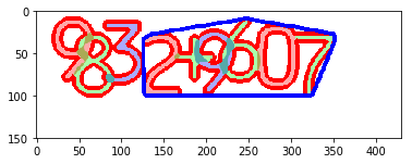
cv2.boundingRect(contour): Contour를 포함하는 사각형을 그립니다.
- 사각형의 X, Y 좌표와 너비, 높이를 반환합니다.
import cv2
import matplotlib.pyplot as plt

image = cv2.imread('Downloads/img.png')
image_gray = cv2.cvtColor(image, cv2.COLOR_BGR2GRAY)
ret, thresh = cv2.threshold(image_gray, 230, 255, 0)

plt.imshow(cv2.cvtColor(thresh, cv2.COLOR_GRAY2RGB))
plt.show()


contours,_ = cv2.findContours(thresh, cv2.RETR_TREE, cv2.CHAIN_APPROX_SIMPLE)
image = cv2.drawContours(image, contours, -1, (0, 255, 0), 4)

plt.imshow(cv2.cvtColor(image, cv2.COLOR_BGR2RGB))
plt.show()


contour = contours[0]
x, y, w, h = cv2.boundingRect(contour)
image = cv2.rectangle(image, (x, y), (x + w, y + h), (0, 0, 255), 3)

plt.imshow(cv2.cvtColor(image, cv2.COLOR_BGR2RGB))
plt.show()


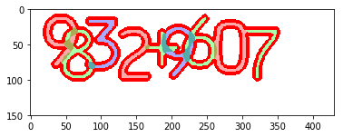
cv2.convexHull(contour): Convex Hull 알고리즘으로 외곽을 구하는 함수
- 대략적인 형태의 Contour 외곽을 빠르게 구할 수 있습니다. (단일 Contour 반환)
import cv2
import matplotlib.pyplot as plt

image = cv2.imread('Downloads/img.png')
image_gray = cv2.cvtColor(image, cv2.COLOR_BGR2GRAY)
ret, thresh = cv2.threshold(image_gray, 230, 255, 0)
thresh = cv2.bitwise_not(thresh)

contours= cv2.findContours(thresh, cv2.RETR_TREE, cv2.CHAIN_APPROX_SIMPLE)[0]
image = cv2.drawContours(image, contours, -1, (0, 0, 255), 4)

plt.imshow(cv2.cvtColor(image, cv2.COLOR_BGR2RGB))
plt.show()

contour = contours[0]
hull = cv2.convexHull(contour)
image = cv2.drawContours(image, [hull], -1, (255, 0, 0), 4)

plt.imshow(cv2.cvtColor(image, cv2.COLOR_BGR2RGB))
plt.show()
cv2.approxPolyDP(curve, epsilon, closed): 근사치 Contour를 구합니다.
- curve: Contour
- epsilon: 최대 거리 (클수록 Point 개수 감소)
- closed: 폐곡선 여부
import cv2
import matplotlib.pyplot as plt

image = cv2.imread('Downloads/img.png')
image_gray = cv2.cvtColor(image, cv2.COLOR_BGR2GRAY)
ret, thresh = cv2.threshold(image_gray, 230, 255, 0)
thresh = cv2.bitwise_not(thresh)

contours = cv2.findContours(thresh, cv2.RETR_TREE, cv2.CHAIN_APPROX_SIMPLE)[0]
image = cv2.drawContours(image, contours, -1, (0, 0, 255), 4)

plt.imshow(cv2.cvtColor(image, cv2.COLOR_BGR2RGB))
plt.show()

contour = contours[0]
epsilon = 0.01 * cv2.arcLength(contour, True)
approx = cv2.approxPolyDP(contour, epsilon, True)
image = cv2.drawContours(image, [approx], -1, (0, 255, 0), 4)

plt.imshow(cv2.cvtColor(image, cv2.COLOR_BGR2RGB))
plt.show()

# 입실론 값 줄일수록 보다 유사 다각형으로-->컨투어 모양이 정확해짐. 커지면-->approximate
cv2.contourArea(contour): Contour의 면적을 구합니다.
cv2.arcLength(contour): Contour의 둘레를 구합니다.
cv2.moments(contour): Contour의 특징을 추출합니다.
import cv2
import matplotlib.pyplot as plt

image = cv2.imread('Downloads/img.png')
image_gray = cv2.cvtColor(image, cv2.COLOR_BGR2GRAY)
ret, thresh = cv2.threshold(image_gray, 230, 255, 0)
thresh = cv2.bitwise_not(thresh)

contours = cv2.findContours(thresh, cv2.RETR_TREE, cv2.CHAIN_APPROX_SIMPLE)[0]
image = cv2.drawContours(image, contours, -1, (0, 0, 255), 4)

contour = contours[0]
area = cv2.contourArea(contour)
print(area)

length = cv2.arcLength(contour, True)
print(length)

M = cv2.moments(contour)
print(M)

plt.imshow(cv2.cvtColor(image, cv2.COLOR_BGR2RGB)))
plt.show()
9637.5
1112.1046812534332 {'m00': 9637.5, 'm10': 2328654.1666666665, 'm01': 525860.6666666666, 'm20': 592439950.25, 'm11': 125395340.54166666, 'm02': 32616659.75, 'm30': 157199366984.05002, 'm21': 31597487112.5, 'm12': 7677332730.433333, 'm03': 2223038890.5, 'mu20': 29780523.227014065, 'mu11': -1665373.5978347063, 'mu02': 3923591.96819859, 'mu30': -339915780.7390442, 'mu21': 76375946.41720533, 'mu12': -21905836.49518633, 'mu03': 15169233.760740757, 'nu20': 0.3206295471760697, 'nu11': -0.01793010748946005, 'nu02': 0.04224302932750429, 'nu30': -0.03727866486560947, 'nu21': 0.008376172780476334, 'nu12': -0.0024024196097321344, 'nu03': 0.001663614382378067}
코드/소스참고: 나동빈
'소프트웨어융합 > 파이썬 기타.py' 카테고리의 다른 글
| 모두의 딥러닝 개정2판 (1) | 2021.10.07 |
|---|---|
| python - opencv: Filtering. KNN (0) | 2021.09.28 |
| python: opencv: 툴이해 기본(1) (0) | 2021.09.27 |
| 2004-2020 변화한 것들.pandas (0) | 2021.09.11 |
| pandas - dataframe 복습 사이트 모음 (1) | 2021.09.08 |

